Importing data into DDModeling is done by calling the function DDRep() which takes two arguments model and raw. model represents a DDModel object (see here for a tutorial). raw specifies the raw data from a given experiment. For a successful import, raw must follow a formatting convention. This convention is examined in the following section.

How to format RAW data

The raw data in the DDModeling package is handled in data.frames, which contain three coulmns:

• cond (factor): Specifies the condition under which a given trial was performed
• resp (numeric): Specifies the binary coded response property of a study
• time (numeric): Indicates the time (in rounded ms) for a given trial

The naming convention within the cond can be chosen freely, but you must ensure that the factor names match the model within the DDRep() function, which means that the conditions specified in the model must match those in your data! resp on the other hand follows a uniform coding scheme: The value 0 represents a trial that led to an error (i.e. wrong answer) and the value 1 represents a trial that led to a success (i.e. correct answer). The time must be given in rounded millisecond (only natural numbers are allowed).

For demonstration purposes, DDModeling comes with a predefined dataset FLANKER_DATA representing 64 datasets (i.e. subjects) of a flanker task experiment with 320 trials per condition. If you want to import data into DDModeling, your data should look like this

library(DDModeling)
#> Lade nötiges Paket: data.table
head(FLANKER_DATA[[1]])
#>     cond time resp
#> 1   Cong  554    1
#> 2 Incong  613    0
#> 3   Cong  833    0
#> 4   Cong  433    1
#> 5   Cong  578    1
#> 6 Incong  439    1

How to import data

After you formatted your data according to the above conventions and constructed an according DDModel importing it is rather simple.

DSTP <- DDModel(model="DSTP",task = "flanker",CDF_perc = c(0.1,0.3,0.5,0.7,0.9), CAF_perc = c(0.0,0.2,0.4,0.6,0.8,1.0))
Subj <- DDRep(model = DSTP,raw = FLANKER_DATA[[1]])

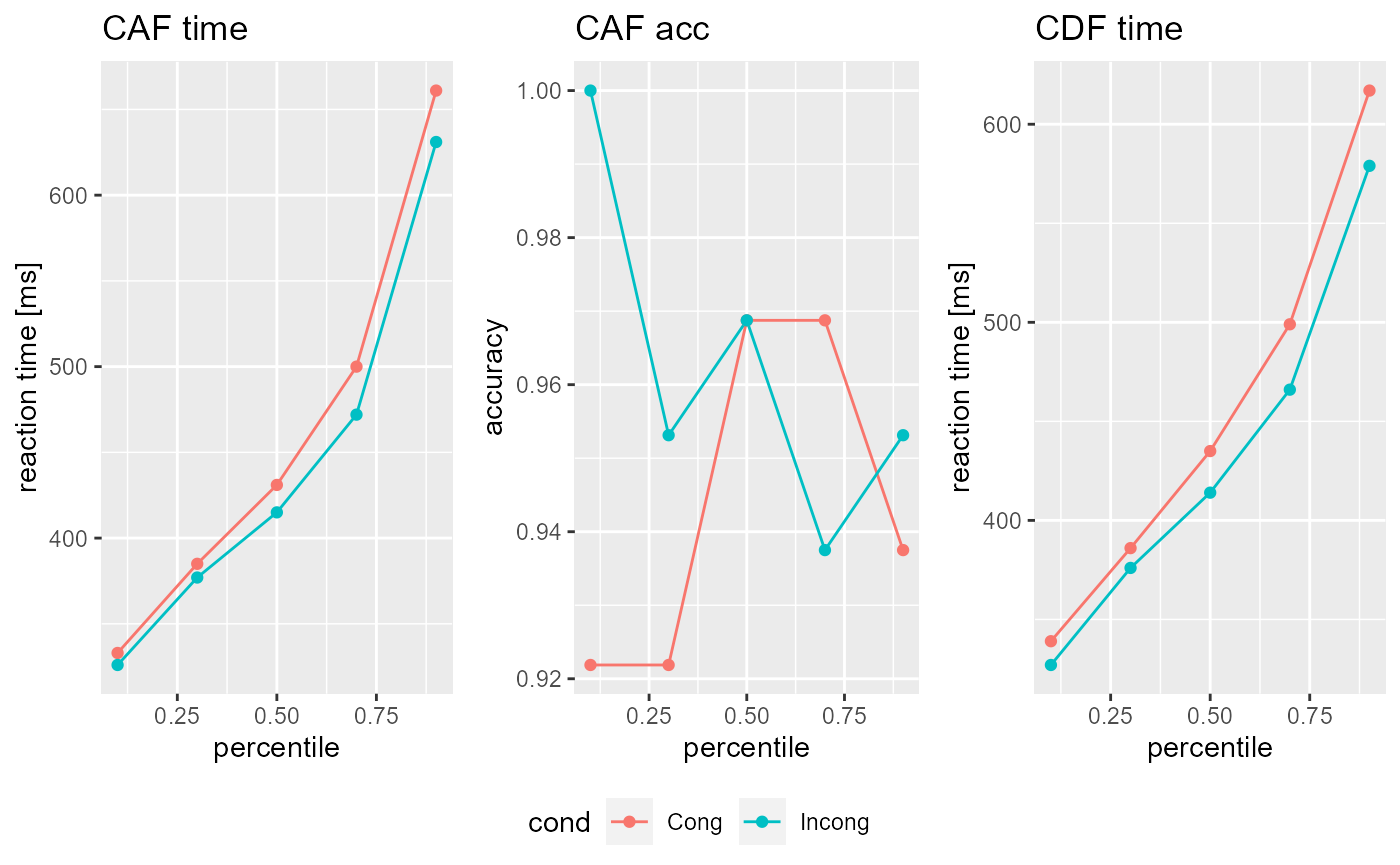
Finally you can take a look at your imported data simply by calling the object or using the plot() function.

Subj
#> CDF: 
#> $Cong
#>   cond perc time   N
#> 1 Cong  0.1  339  30
#> 2 Cong  0.3  386  90
#> 3 Cong  0.5  435 151
#> 4 Cong  0.7  499 211
#> 5 Cong  0.9  617 271
#> 
#> $Incong
#>     cond perc time   N
#> 1 Incong  0.1  327  30
#> 2 Incong  0.3  376  92
#> 3 Incong  0.5  414 154
#> 4 Incong  0.7  466 215
#> 5 Incong  0.9  579 277
#> 
#> 
#> CAF: 
#> $Cong
#>   cond perc time      acc N_A N_B
#> 1 Cong  0.1  333 0.921875  59   5
#> 2 Cong  0.3  385 0.921875  59   5
#> 3 Cong  0.5  431 0.968750  62   2
#> 4 Cong  0.7  500 0.968750  62   2
#> 5 Cong  0.9  661 0.937500  60   4
#> 
#> $Incong
#>     cond perc time      acc N_A N_B
#> 1 Incong  0.1  326 1.000000  64   0
#> 2 Incong  0.3  377 0.953125  61   3
#> 3 Incong  0.5  415 0.968750  62   2
#> 4 Incong  0.7  472 0.937500  60   4
#> 5 Incong  0.9  631 0.953125  61   3
#> 
#> 
#> Parameter: 
#>   Ter a c mu_t mu_f mu_RS2 mu_SS
#> 1   0 0 0    0    0      0     0
plot(Subj)